This is the second installment in our series to educate our readers on the time-saving and resource-maximizing capabilities of Microsoft Excel. Gaining Excel tricks can yield huge productivity rewards and allow you to manipulate and calculate more effectively and thoroughly than ever before.
Click here if you missed Part I
What we’ve covered so far…
- Use a template
- COUNT and SUM functions
- Keyboard shortcuts
- Auto-Fill
- Inserting rows or columns
6. Filter Your Data
At times you likely prefer to just look at a portion of your data and not the whole raw spreadsheet. Never worry- filtering exists and it will allow you to pare down to a subset of that data quickly.
AutoFilter is the easiest first lesson in filtering in Excel.
Try this: Highlight the row containing your column headings, then navigate to the “Data” tab on your excel top menu and choose “Filter”. Excel will have determined the fields populating each column and now with each heading you can sort down that column by the various contents that appeared under each heading. You can also filter out blank cells, sort alphabetically, and other such organizational steps.
7. Freeze A Row or Column
This will allow you to scroll all over your worksheet (far down or far across) while keeping rows or columns to the top or right visible at all times.
On Excel’s “View” tab you will see a few different freeze pane options. Aside from easily freezing the top row or right column, the third option is to select multiple to stick to the top or right while you scroll.
When you highlight a row and click “Freeze panes”, anything to the left of it will freeze and the row you highlighted will be the first of the rest of the worksheet to move. The same rule applies to columns.
8. Define A Print Area
On the “Page Layout” tab, under “Page Setup”, you can click “Print Area” and “Select Print Area”. This will allow you to manipulate what gets printed when you select “Print” at the end of your work, and in this process you can determine where and how your pages get cut off.
9. Protect With A Password
When you go to save your document, choose “Save As” and navigate to the “Tools” button. There you will see “General Options”. Here you can designate a password that will protect your spreadsheet from being opened by anyone without the password. This is especially helpful in the case that you’re working with personal health information, financial data, and other scenarios of this level of sensitivity.
10. Create Multiple Worksheets
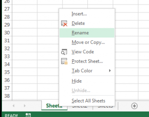
Each Excel workbook (excel file you create is a “workbook”) starts out with 3 tabs, or “worksheets”- Sheet1, Sheet2, and Sheet3. You can rename these, add or reduce the number of worksheets, and work off of multiple worksheets in your workbook.
To rename or delete a worksheet, just right click the tab to be given your options.

You can drag worksheet tabs across each other to reorder them. You can add more by clicking the plus (+) circle or the new sheet icon in the case that you’re using an older version of Excel.
![]()
This concludes the 2nd in our series of 20 Easy Tips For Using Microsoft Excel.
Ready for more?:
—
In the meantime, we want to hear from you. What questions can we answer? What challenges are you looking to address for your business or yourself?
