This is the third in our series covering some easy Excel tricks to make this program work for you. Learning some of these can save you time and give you cleaner, better, more meaningful results.
Click here for Tips 1-5
Click here for Tips 6-10
What we’ve covered so far…
- Use a template
- COUNT and SUM functions
- Keyboard shortcuts
- Auto-Fill
- Inserting rows or columns
- Filter your data
- Freeze a row or column
- Define a print area
- Protect with a password
- Create multiple worksheets
11. Visualize Your Data
Make your data stand out and make it friendlier to readers: Put it all into a sort of visual map for readers to navigate the data more easily!
Highlight the data you want to make into a chart or graph. Then, go to “Insert” and find “Charts”. You can take a recommendation from Excel or start with your favorite visualizations.
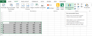
For more advanced users: You’ll also find pivot table and pivot chart options in this section of the menu!
12. Select Your Entire Worksheet With One Click
On the top left corner of your spreadsheet, between row 1 and column A labels, there’s a little corner arrow.
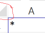
Click it, and your entire sheet will be highlighted. Ta-dah!
13. Edit Cell Borders
You can put borders around individual cells or bulk areas of your spreadsheet. This particular tool will also let you create diagonal lines across cells if you’d like. You can select the thickness or pattern of the lines that make up your borders. Right-click the area you want to border and choose “Format Cells…”. Border options is the 4th tab across under Format Cells. Take a look to explore your options.
14. Transpose Data from Rows to Columns
Sometimes, especially if you’re exporting from data collection resources, data is difficult to read because it populates rows when you need to see it in columns or vice versa.
There is a way to paste data after you copy it that allows you to switch from having it in many rows to having it in columns. First, copy whatever data on your sheet you want to shift from being in rows to being in columns. If you have headers for your rows or columns, include them in the copied area.
From there, go to your home tab of your top menu bar, and navigate to “Paste”. Choose “Transpose”. If you don’t see “Transpose” or it’s grayed out, make sure you highlighted and copied your data first! If you don’t, it won’t be an option.
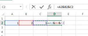
15. Combine Contents of Multiple Cells Into One Cell
There is a “concatenate” function to use for this, but we are going to tell you the “easy” way instead: Just use the ampersand (“&”) in your function in between cells!
This concludes the 3rd in our series of 20 Easy Tips For Using Microsoft Excel.
We want to hear from you. What questions can we answer?
What challenges are you looking to address for your business or yourself?